Chap. 2

Functional Analysis

My Intuitive Overview of Functional Analysis (a draft)

What is functional analysis ?

Functional analysis seems to extend the concepts of Algebra into infinite-dimensional spaces. It is actually a blend of Algebra and Topology, more particularly, it is the extension of Linear Algebra, since Linear Algebra is the most studied subject of algebra. But what exactly does functional analysis aim to do?

It focuses on the study of topological vector spaces and the maps between them, with some additional algebraic and topological conditions’ assumptions on these maps.
It explores infinite-dimensional spaces, where functions themselves become the primary objects of study. This shift was imposed because many problems in analysis, differential equations, and physics naturally lead us to consider spaces of functions, which can’t be adequately described using finite-dimensional methods.

For example …

Continuous functions on $[0, 1]$

A function space, such as $C ([0, 1])$ , the space of continuous functions on $[0, 1]$ , or $L^{2} ([0, 1])$ , square-integrable functions, cannot be spanned by a finite set of functions.

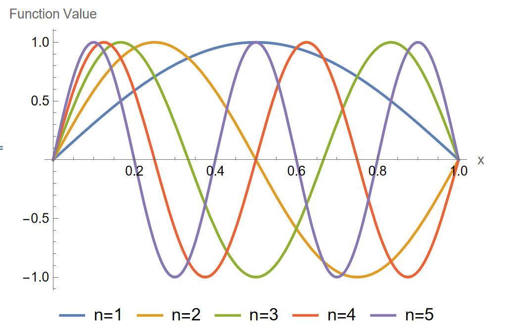
Orthogonal elements from a basis in $L^{2} ([0, 1])$ , using sine functions from Fourier analysis look like :

Each curve $\sin (n π x)$ is orthogonal to the others under the inner product: $⟨ f, g ⟩ = \int_{0}^{1} f (x) g (x) d x .$

No finite subset of these functions can describe all possible functions in $L^{2} ([0, 1])$ .

Delay Differential Equation (DDE)

A standard Ordinary Differential Equation (ODE) like:

\frac{d y}{d t} = - y (t)

defines the future state $y (t)$ based solely on its current value $y (t)$ . If you know $y (t_{0})$ at some initial time $t_{0}$ , you can compute $y (t)$ for all $t > t_{0}$ without needing additional information.

In contrast, a Delay Differential Equation (DDE) like:

\frac{d y}{d t} = - y (t) + y (t - τ)

requires the value of $y (t - τ)$ - the state of the system at a previous time - to compute the future state $y (t)$ .

This means that to solve the equation, you need to know $y (t)$ for all times $t$ in the interval $[t_{0} - τ, t_{0}]$ .

The system now depends on an entire function (the history of $y$ ), not just a single value.

The dependency on $y (t - τ)$ means that the state of the system at any time $t$ is described not by a single number (as in ODEs) but by a function defined over the interval $[t - τ, t]$ . This function contains infinitely many pieces of information (its values at infinitely many points), which cannot be encoded by a finite number of parameters.

In mathematical terms:

For an ODE, the state space is finite-dimensional because it is sufficient to specify the values of $y (t)$ and possibly its derivatives at a single point $t_{0}$ .
For a DDE, the state space is infinite-dimensional because the system’s future evolution depends on the entire function $y (t)$ over the interval $[t - τ, t]$ .

The space of polynomials

The space of all polynomials is infinite-dimensional. A finite basis fails because for any largest degree $n$ , adding a polynomial of degree $n + 1$ would exceed the basis, highlighting the necessity of infinite bases.

The space of square-integrable functions $L^{2} ([0, 1])$

The space $L^{2} ([0, 1])$ consists of all functions $f (x)$ defined on the interval $[0, 1]$ such that:

\int_{0}^{1} | f (x) |^{2} d x < \infty .

This space is infinite-dimensional for the following reasons:

Consider the set of orthogonal functions ${e_{n} (x) = \sin (n π x), \cos (n π x)}$ for $n =$ $1, 2, 3, \dots$ . These functions are linearly independent and there’s an infinite number of them, meaning none of them can be expressed as a finite linear combination of the others.

Suppose $L^{2} ([0, 1])$ had a finite basis of $m$ functions ${f_{1}, f_{2}, \dots, f_{m}}$ . Any function in $L^{2} ([0, 1])$ would then have to be expressed as a linear combination of these $m$ basis functions:

f (x) = c_{1} f_{1} (x) + c_{2} f_{2} (x) + \dots + c_{m} f_{m} (x) .

But, there exist infinitely many orthogonal functions (e.g., the Fourier basis). Adding one more orthogonal function to the set would produce a contradiction, as it could not be expressed in terms of the finite basis.

So, how do we handle these infinite dimensions?

This brings us to the hierarchy of spaces in functional analysis:

Topological spaces: At the foundation, we have topological spaces, which introduce the notion of open sets, and in turn discuss “closeness” without necessarily defining a distance or a way to measure closeness.

This allows us to frame the more general notion of convergence of sequences, which will depend on the chosen topology. So, by changing topology, we change the way we converge, because we would change the way we frame elements (classes) in sets and how to distinguish between them. So different types of topologies, will provide different types of convergence (weak, weak*, strong) with different properties.
Metric spaces: By introducing a metric, we obtain metric spaces where we can measure distances between points. This is useful for defining concepts like the Contraction Mapping Principle and fixed-point theorems, which help proving the existence and uniqueness of solutions to equations such as ODEs. These concepts have applications in dynamical systems, where understanding the behavior of solutions over time is essential.
Normed spaces: Introducing a norm assigns a length to each vector, generalizing the absolute value on real numbers or the Euclidean norm in finite-dimensional spaces. Norms help us quantify the size of functions. In normed spaces, we can define dual spaces and study linear functionals, leading to concepts like weak convergence and optimization in these spaces.
Banach spaces: When a normed space is complete—meaning every Cauchy sequence converges within the space—we have a banach space. Banach spaces are fundamental because they provide the setting for many powerful theorems:
- The Hahn-Banach Theorem allows the extension of linear functionals and underpins duality principles in optimization.
- The Banach-Steinhaus Theorem, or Uniform Boundedness Principle, ensures the stability of sequences of bounded operators.
- The Open Mapping Theorem and Closed Graph Theorem help us understand the behavior of linear operators, crucial for solving operator equations.

These theorems have practical implications in solving integral equations and understanding the continuity and surjectivity of operators in functional spaces.

Inner product spaces: By introducing an inner product, we can talk about angles and orthogonality between vectors. This leads to the Projection Theorem, fundamental in approximation theory and methods like the least squares approximation used in data fitting and regression analysis. These concepts are widely used in statistics and machine learning for modeling and data analysis.
Hilbert spaces: When an inner product space is complete, we obtain a Hilbert space. Hilbert spaces are the playground for much of functional analysis, especially in areas like:
- Fourier series and transforms: essential for signal processing and communication systems, allowing us to decompose functions into frequencies.
- The spectral theorem: provides tools for studying linear operators, leading to applications in quantum mechanics and quantum computing.
- Weak Formulation of PDEs: By considering weak solutions, we can handle PDEs that may not have classical solutions, using methods like the Galerkin Method and Finite Element Method (FEM) for numerical approximations, which are used in engineering simulations.

But dealing with infinite-dimensional spaces isn’t without challenges. Solutions to equations in these spaces might not exist in the traditional sense or might not be unique. This leads us to the concept of weak or very weak solutions. By relaxing the requirements of a solution, we can find functions that satisfy the equations in an averaged or generalized sense. This is particularly common in fields like fluid dynamics, where classical solutions to the Euler or Navier-Stokes equations might be difficult to find or prove to be unique. So, what guarantees uniqueness in these cases?

Questions about existence and uniqueness often lead to open problems. For example, the uniqueness of solutions to the Navier-Stokes equations is one of the Millennium Prize Problems.

Researchers explore conditions, like entropy conditions, that might ensure uniqueness or stability of solutions.

When solutions exist, we often need to find them numerically. Infinite-dimensional problems are impossible to compute directly, so we use numerical methods to approximate them with finite-dimensional ones.

Methods like the Finite Element Method and the Galerkin Method discretize the problem, reducing it to solving large but sparse linear systems.

Here, functional analysis provides the theoretical foundation to study:

Convergence: Do these approximations converge to the true solution? If so, how fast?

$\to$ Understanding the rate of convergence helps in assessing the efficiency of numerical methods.
Computational Complexity: What are the time and memory requirements?

$\to$ Since we can choose how to implement these methods, analyzing complexity helps in optimizing performance.
Stability: Are the solutions stable under small perturbations?

$\to$ Functional analysis helps us understand the stability of numerical schemes, which is crucial for reliable simulations.

At the core of these analyses is the need to develop notions of convergence of sequences of functions and to study their properties.

The concept of convergence depends on the structure of the space

Topological spaces: It’s enough to have the notion of open sets to discuss convergence.
Metric spaces: A metric allows us to define the distance between functions, giving a more precise notion of convergence.
Normed spaces: Norms generalize the concept of length, enabling us to measure the size of functions.
Inner product spaces: With inner products, we can define angles and orthogonality, leading to projections and optimization methods.

For example, in optimization and approximation, if a solution lies outside the feasible region, we can project it onto the feasible set, finding the closest point within the constraints. This projection relies on the geometric structure provided by inner product spaces.

In summary, functional analysis builds a hierarchy of spaces:

Inner product spaces (angles) ⊂ Normed spaces (length) ⊂ Metric spaces (distance) ⊂ Topological spaces (open sets)

Each level adds structure, enabling us to tackle increasingly complex problems. By understanding these spaces and the relationships between them, we gain the tools necessary to address infinite-dimensional problems that arise in various fields.

By building upon each level of structure, we can understand and solve problems that would otherwise be intractable.

--- theme: default --- graph TD A[Functional Analysis] %% Hierarchy of Spaces A --> B[Topological Spaces] B --> C[Metric Spaces] C --> D[Normed Spaces] D --> E[Banach Spaces] D --> F[Inner Product Spaces] F --> G[Hilbert Spaces] %% From Topological Spaces B --> H[Continuous Functions] H --> I[Compactness and Connectedness] I --> J[Topological Invariants] J --> K[Algebraic Topology] K --> L[Applications in Geometry] %% From Metric Spaces C --> M[Contraction Mapping Principle] M --> N[Fixed-Point Theorems] N --> O[Existence and Uniqueness of Solutions to ODEs] O --> P[Applications in Dynamical Systems] %% From Normed Spaces D --> Q[Dual Spaces] Q --> R[Linear Functionals] R --> S[Weak Convergence] S --> T[Optimization in Normed Spaces] %% From Banach Spaces E --> U[Hahn-Banach Theorem] U --> V[Extension of Linear Functionals] V --> W[Duality Principles] W --> X[Optimization Theory] E --> Y[Banach-Steinhaus Theorem] Y --> Z[Uniform Boundedness Principle] Z --> AA[Stability of Functional Equations] E --> AB[Open Mapping Theorem] AB --> AC[Surjectivity of Bounded Operators] AC --> AD[Inverse Mapping Theorem] AD --> AE[Solving Operator Equations] E --> AF[Closed Graph Theorem] AF --> AG[Continuity of Operators] AG --> AH[Functional Equations in Banach Spaces] %% From Inner Product Spaces F --> AI[Orthogonality] AI --> AJ[Projection Theorem] AJ --> AK[Least Squares Approximation] AK --> AL[Data Fitting and Regression] %% From Hilbert Spaces G --> AM[Fourier Series and Transforms] AM --> AN[Signal Processing] AN --> AO[Communication Systems] G --> AP[Spectral Theorem] AP --> AQ[Quantum Mechanics] AQ --> AR[Quantum Computing] G --> AS[Weak Formulation of PDEs] AS --> AT[Variational Methods] AT --> AU[Finite Element Method] AU --> AV[Engineering Simulations] %% Numerical Methods from Hilbert Spaces G --> AW[Galerkin Method] AW --> AU %% Additional Connections AK --> O AU --> AE AQ --> AT %% Removed Redundant Nodes %% Applications are now directly connected through specific theorems and concepts.